Random Forest In R

Random Forest In R

There are laws which demand that the decisions made by models used in issuing loans or insurance be explainable. The latter is known as model interpretability and is one of the reasons why we see random forest models being used over other models like neural networks.

Algorithm

The random forest algorithm works by aggregating the predictions made by multiple decision trees of varying depth. Every decision tree in the forest is trained on a subset of the dataset called the bootstrapped dataset.

The portion of samples that were left out during the construction of each decision tree in the forest are referred to as the Out-Of-Bag (OOB) dataset. As we’ll see later, the model will automatically evaluate its own performance by running each of the samples in the OOB dataset through the forest.

Recall how when deciding on the criteria with which to split a decision tree, we measured the impurity produced by each feature using the Gini index or entropy. In random forest, however, we randomly select a predefined number of feature as candidates. The latter will result in a larger variance between the trees which would otherwise contain the same features (i.e those which are highly correlated with the target label).

When the random forest is used for classification and is presented with a new sample, the final prediction is made by taking the majority of the predictions made by each individual decision tree in the forest. In the event, it is used for regression and it is presented with a new sample, the final prediction is made by taking the average of the predictions made by each individual decision tree in the forest.

R Code

In the proceeding tutorial, we’ll use the caTools package to split our data into training and tests sets as well as the random forest classifier provided by the randomForest package.

library(randomForest)

require(caTools)

We’ll be be working with one of the available datasets from the UCI Machine Learning Repository. If you’d like to follow along, the data can be found here.

Our goal will be to predict whether a person has heart disease given

data <- read.csv(  
  "processed.cleveland.data",  
  header=FALSE  
)

The csv file contains 303 rows and 14 columns.

dim(data)

According to the documentation, the mapping of columns and features is as follows.

1. age: age in years
2. sex: sex (1 = male; 0 =female)
3. cp: chest pain type (1 = typical angina; 2 = atypical angina; 3 = non-anginal pain; 4 = asymptomatic)
4. trestbps: resting blood pressure (in mm Hg on admission to the hopsital)
5. choi: serum cholestoral in mg/dl
6. fbs: fasting blood sugar > 120 mg/dl (1 = true; = 0 false)
7. restecg: resting electrocardiographic results (1 = normal; 2 = having ST-T wave abnormality; 2 = showing probable or definite left ventricular hypertrophy)
8. thalach: maximum heart rate achieved
9. exang: exercise induced angina (1 = yes; 0 = no)
10. oldpeak: ST depression induced by exercise relative to rest
11. slope: the slope of the peak exercise ST segment (1 = upsloping; 2 = flat; 3 = downsloping)
12. ca: number of major vessels (0–3) colored by flourosopy
13. thai: (3 = normal; 6 = fixed defect; 7 = reversable defect)
14. num: diagnosis of heart disease. It is an integer valued from 0 (no presence) to 4.

Given that the csv file does not contain the header, we must specify the column names manually.

names(data) <- c("age", "sex", "cp", "trestbps", "choi", "fbs", "restecg", "thalach", "exang", "oldpeak", "slope", "ca", "thai", "num")

Often times, when we’re working with large datasets, we want to get a sense of our data. As opposed to loading everything in RAM, we can use the head function to view the first few rows.

head(data)

To simplify the problem, we’re only going to attempt to distinguish the presence of heart disease (values 1,2,3,4) from absence of heart disease (value 0). Therefore, we replace all labels greater than 1 by 1.

data$num[data$num > 1] <- 1

R provides a useful function called summary for viewing metrics related to our data. If we take a closer look, we’ll notice that it provides the mean for what should be categorical variables.

summary(data)

This implies that there is an issue with the column types. We can view the type of each column by running the following command.

sapply(data, class)

In R, a categorical variable (a variable that takes on a finite amount of values) is a factor. As we can see, sex is incorrectly treated as a number when in reality it can only be 1 if male and 0 if female. We can use the transform method to change the in built type of each feature.

data <- transform(  
  data,  
  age=as.integer(age),  
  sex=as.factor(sex),  
  cp=as.factor(cp),  
  trestbps=as.integer(trestbps),  
  choi=as.integer(choi),  
  fbs=as.factor(fbs),  
  restecg=as.factor(restecg),  
  thalach=as.integer(thalach),  
  exang=as.factor(exang),  
  oldpeak=as.numeric(oldpeak),  
  slope=as.factor(slope),  
  ca=as.factor(ca),  
  thai=as.factor(thai),  
  num=as.factor(num)  
)

sapply(data, class)

If we, again, print a summary of our data, we get the following.

summary(data)

Now, the categorical variables are expressed as the counts for each respective class. The ca and thai of certain samples are ? indicating missing values. R expects missing values to be written as NA. After replacing them, we can use the colSums function to view the missing value counts of each column.

data[ data == "?"] <- NA

colSums(is.na(data))

According to the notes from above, thai and ca are both factors.

• thai: (3 = normal; 6 = fixed defect; 7 = reversable defect)
• ca: number of major vessels (0–3) colored by flourosopy

I don’t claim to be a domain expert, so we’re just going to replace the missing values for thai with what is considered normal. Next, we’re going to drop the rows where ca is missing.

data$thai[which(is.na(data$thai))] <- as.factor("3.0")  
data <- data[!(data$ca %in% c(NA)),]

colSums(is.na(data))

If we run summary again, we’ll see that it still views ? as a potential class.

summary(data)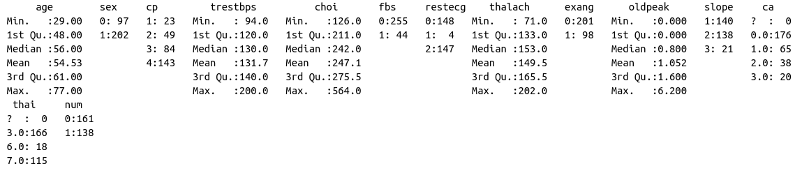

To get around this issue, we cast the columns to factors.

data$ca <- factor(data$ca)  
data$thai <- factor(data$thai)

summary(data)

We’re going to set a portion of our data aside for testing.

sample = sample.split(data$num, SplitRatio = .75)

train = subset(data, sample == TRUE)  
test  = subset(data, sample == FALSE)

dim(train)  
dim(test)

Next, we initialize an instance of the randomForest class. Unlike scikit-learn, we don’t need to explicily call the fit method to train our model.

rf <- randomForest(  
  num ~ .,  
  data=train  
)

By default, the number of decision trees in the forest is 500 and the number of features used as potential candidates for each split is 3. The model will automatically attempt to classify each of the samples in the Out-Of-Bag dataset and display a confusion matrix with the results.

Now, we use our model to predict whether the people in our testing set have heart disease.

pred = predict(rf, newdata=test[-14])

Since this is a classification problem, we use a confusion matrix to evaluate the performance of our model. Recall that values on the diagonal correspond to true positives and true negatives (correct predictions) whereas the others correspond to false positives and false negatives.

cm = table(test[,14], pred)