Decision Tree In Python

Decision Tree In Python

In my opinion, Decision Tree models help highlight how we can use machine learning to enhance our decision making abilities. We’ve all encountered Decision Trees at one point or another. However, where Decision Tree machine learning models differ is in the fact that they use logic and math to generate rules, rather than selecting them on the basis of intuition and subjectivity.

Algorithm

When attempting to build a decision tree, the question that should immediately come to mind is:

On what basis should we make decisions?

In other words, what should we select as the yes or no questions which are used to classify our data. We could take an educated guess (i.e. all mice with a weight over 5 pounds are obese). However, it isn’t necessarily the best way to categorize our samples. What if, we could use some kind of machine learning algorithm to learn what questions to ask in order to do the best job at classifying our data? That is the purpose behind decision tree models.

Suppose that we were trying to build a decision tree to predict whether a person is married. Therefore, we went around the neighborhood knocking on people’s doors and politely asked them to provide their age, sex and income for our little research project. Out of the couple thousand people we asked, 240 didn’t slam the door into our face.

Now, before we continue it’s important that we grasp the following terminology. The top of the tree (or bottom depending on how you look at it) is called the root node. Intermediate nodes have arrows pointing to and away from them. Finally, the nodes at the bottom of the tree without any edges pointing away from them are called leaves. Leaves tell you what class each sample belongs to.

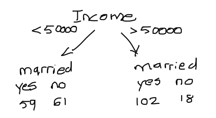
Going back to our example, we need to figure out how to go from a table of data to a decision tree. Rather than selecting the branches ourselves, we decide to use a machine learning algorithm to construct the decision tree for us. The model looks at how well each feature separates people who are and aren’t married. Since income is a continuous variable, we set an arbitrary value.

In order to determine which of the three splits is better, we introduce a concept called impurity. Impurity refers to the fact that none of the leaves have a 100% “yes married”. There are several ways to measure impurity (quality of a split), however, the scikit-learn implementation of the DecisionTreeClassifer uses gini by default, therefore, that’s the one we’re going to cover in this article.

To calculate the Gini impurity of the left leaf, we subtract 1 by the fraction of people that are married squared and the fraction of people that aren’t married squared.

The equation is the exact same for the impurity of the right leaf.

The Gini impurity for the node itself is 1 minus the fraction of samples in the left child, minus the fraction of samples in the right child.

The information gain (with Gini Index) is written as follows.

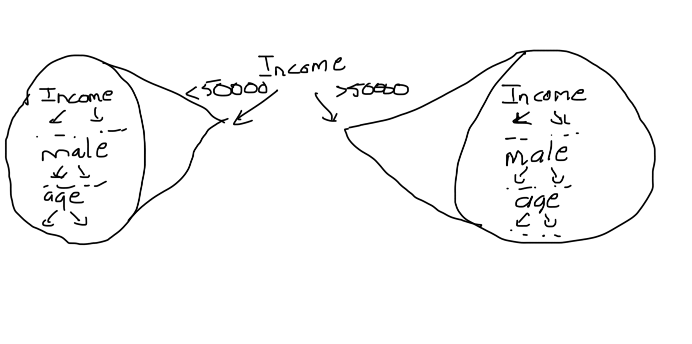
The process is then repeated for income and sex. We ultimately decide on the split with the largest information gain. In this case, it’s income, which makes sense since there is a strong correlation between an income of greater than 50,000 and being married. If we ask that question right away, we make a substantial leap towards correctly classifying our data.

Once we’ve decided on the root, we repeat the process for the other nodes in the tree. It’s worth noting that:

a) We can split on income again

b) The number of samples in each branch can differ

We can’t go on splitting indefinitely. Therefore, we need a way of telling the tree when to stop. The scikit-learn implementation of the DecisionTreeClassifer uses the minimum impurity decrease to determine whether a node should be split.

Suppose that we after a few more iterations, we end up with the following node on the left hand side of the tree.

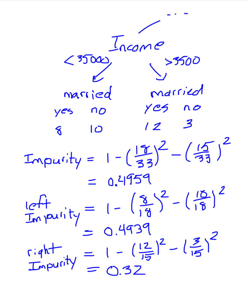
The result is greater than the default threshold of 0. Therefore, the node will be split. Had it been below 0, the node’s children would have been considered a leaves.

Python Code

Let’s take a look at how we could go about implementing a decision tree classifier in Python. To begin, we import the following libraries.

from sklearn.datasets import load_iris  
from sklearn.tree import DecisionTreeClassifier  
from sklearn.model_selection import train_test_split  
from sklearn.metrics import confusion_matrix  
from sklearn.tree import export_graphviz  
from sklearn.externals.six import StringIO   
from IPython.display import Image   
from pydot import graph_from_dot_data  
import pandas as pd  
import numpy as np

For this tutorial, we’ll be working with what has to be the most popular dataset in the field of machine learning, the iris dataset from UC Irvine Machine Learning Repository.

iris = load_iris()  
X = pd.DataFrame(iris.data, columns=iris.feature_names)  
y = pd.Categorical.from_codes(iris.target, iris.target_names)

In the proceeding section, we’ll attempt to build a decision tree classifier to determine the kind of flower given its dimensions.

X.head()

Although, decision trees can handle categorical data, we still encode the targets in terms of digits (i.e. setosa=0, versicolor=1, virginica=2) in order to create a confusion matrix at a later point. Fortunately, the pandas library provides a method for this very purpose.

y = pd.get_dummies(y)

We’ll want to evaluate the performance of our model. Therefore, we set a quarter of the data aside for testing.

X_train, X_test, y_train, y_test = train_test_split(X, y, random_state=1)

Next, we create and train an instance of the DecisionTreeClassifer class. We provide the y values because our model uses a supervised machine learning algorithm.

dt = DecisionTreeClassifier()

dt.fit(X_train, y_train)

We can view the actual decision tree produced by our model by running the following block of code.

dot_data = StringIO()

export_graphviz(dt, out_file=dot_data, feature_names=iris.feature_names)

(graph, ) = graph_from_dot_data(dot_data.getvalue())

Image(graph.create_png())

Notice how it provides the Gini impurity, the total number of samples, the classification criteria and the number of samples on the left/right sides.

Let’s see how our decision tree does when its presented with test data.

y_pred = dt.predict(X_test)

If this were a regression problem, we’d use some kind of loss function such as Mean Square Error (MSE). However, since this is a classification problem, we make use of a confusion matrix to gauge the accuracy of our model. The confusion matrix is best explained with the use of an example.

Suppose your friend just took a pregnancy test. The results could fall in one of the 4 following categories.

True Positive:

Interpretation: You predicted positive and it’s true.

You predicted that a woman is pregnant and she actually is.

True Negative:

Interpretation: You predicted negative and it’s true.

You predicted that a man is not pregnant and he actually is not.

False Positive: (Type 1 Error)

Interpretation: You predicted positive and it’s false.

You predicted that a man is pregnant but he actually is not.

False Negative: (Type 2 Error)

Interpretation: You predicted negative and it’s false.

You predicted that a woman is not pregnant but she actually is.

That being said, the numbers on the diagonal of the confusion matrix correspond to correct predictions. When there are more than two potential outcomes, we simply extend the number of columns and rows in the confusion matrix.

species = np.array(y_test).argmax(axis=1)  
predictions = np.array(y_pred).argmax(axis=1)  
confusion_matrix(species, predictions)

As we can see, our decision tree classifier correctly classified 37/38 plants.

Conclusion

Decision Trees are easy to interpret, don’t require any normalization, and can be applied to both regression and classification problems. Unfortunately, Decision Trees are seldom used in practice because they don’t generalize well. Stay tuned for the next article where we’ll cover Random Forest, a method of combining multiple Decision Trees to achieve better accuracy.