Machine Learning Algorithms Part 5: Random Forest Classification In Python

Machine Learning Algorithms Part 5: Random Forest Classification In Python

The random forest algorithm makes use of multiple decision trees. It can solve both regression and classification problems. With Random Forest however, learning may be slow (depending on the parameterization) and it is not possible to iteratively improve the generated models.

Random Forest can be used in real-world applications such as:

• Predict patients for high risks
• Predict parts failures in manufacturing
• Predict loan defaulters

As mentioned previously, at the heart of the random forest algorithm are decision trees. Suppose we wanted to sort a bucket of fruit into distinct categories. We could start off by asking a question that would only hold true for one kind of fruit. The others would subsequently be placed in a new bucket. We repeat the process until all the fruit is classified.

When we encounter a new fruit, we could predict its type by tracing through the decision tree, always picking the path corresponding to that fruit’s characteristics.

Decision trees leave you with a difficult decision. A deep tree with lots of leaves will overfit whereas a shallow tree with few leaves will perform poorly because it fails to capture as many distinctions in the raw data.

The random forest algorithm uses many trees. It makes a prediction by taking the majority of the predictions made by each component tree. It generally has much better predictive accuracy than a single decision tree.

Going back to our example, imagine our model was tasked with classifying a new mystery fruit. Every decision tree would independently come up with an answer as to where they think it should go. The random forest algorithm would then categorize the fruit by a rule of majority.

Let’s take a look at how we could go about classifying data using the random forest algorithm with python. For this tutorial, we’ll be using a data set containing 3 classes of 50 instances each, where each class refers to a type of iris plant.

from sklearn.datasets import load_iris

from sklearn.ensemble import RandomForestClassifier

from sklearn.model_selection import train_test_split

from sklearn.metrics import confusion_matrix

import pandas as pd

import numpy as np

We can easily load the data into our program using the sklearn.datasets module.

iris = load_iris()

X = pd.DataFrame(iris.data, columns=iris.feature_names)

y = pd.Categorical.from_codes(iris.target, iris.target_names)

We must encode categorical data (i.e. names of flours) for it to be interpreted by the model. In one hot encoding, the class is determined by the location of the number 1. For example, you’d represent a setosa as [1, 0, 0] and versicolor as [0, 1, 0].

one_hot_encoded_y = pd.get_dummies(y)

The point of building a model, is to classify new data. Therefore, we need to put aside data to verify whether our model does a good job at predicting new incoming data or it is overfitting. By default, the test set created by train_test_split is 25% of the original data.

Many machine learning models allow some randomness in model training. Specifying a number for random_state ensures you get the same results in each run. This is considered a good practice. You use any number, and model quality won’t depend meaningfully on exactly what value you choose.

train_X, val_X, train_y, val_y = train_test_split(X, y, random_state=1)

The sklearn library has already taken care of the random forest algorithm implementation. To use it, we create an instance of RandomForestClassifier.

rf_model = RandomForestClassifier()

In the context of machine learning, fit is synonymous with train. Random forest is supervised machine learning algorithm because we feed the model correctly labeled data (train_y) during the training process.

rf_model.fit(train_X, train_y)

Using our newly trained model, we predict the classes given the features in the test set.

rf_val_predictions = rf_model.predict(val_X)

If this were a regression problem, we’d use some kind of loss function but in classification problems, we make use of the confusion matrix determine the accuracy of our model.

Suppose your friend just took a pregnancy test. The results can fall in one of the 4 following categories.

True Positive:

Interpretation: You predicted positive and it’s true.

You predicted that a woman is pregnant and she actually is.

True Negative:

Interpretation: You predicted negative and it’s true.

You predicted that a man is not pregnant and he actually is not.

False Positive: (Type 1 Error)

Interpretation: You predicted positive and it’s false.

You predicted that a man is pregnant but he actually is not.

False Negative: (Type 2 Error)

Interpretation: You predicted negative and it’s false.

You predicted that a woman is not pregnant but she actually is.

That being said, the numbers on the diagonal of the confusion matrix correspond to correct predictions. Before we can create the confusion matrix, we must encode the targets in terms of digits (i.e. setosa=0, versicolor=1, virginica=2).

species = np.array(val_y).argmax(axis=1)  
predictions = np.array(rf_val_predictions).argmax(axis=1)

confusion_matrix(species, predictions)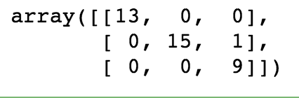

As you can see, our model has an accuracy of 37/38 = 97.3%.

Cory Maklin
_Sign in now to see your channels and recommendations!_www.youtube.com